Examples

Learning by means of examples

In this document some examples for each type of analysis is given. Working codes of the presented examples are included in the SpicePy repo (folder demo). All those interested only in the examples can download them here.

DC network

Let us consider the network in the following figure,

it is described by the file network.net including the following lines:

* Example of DC network
R2 1 2 5 
R1 1 3 10
V2 2 0 15
V1 3 0 5 
I1 2 1 2 
R3 1 0 2 
.op

Please note that elements are intentionally included without a fixed order because it not required any specific sequence.

The network can be solved executing the following python code:

# import SciPy modules
import spicepy.netlist as ntl
from spicepy.netsolve import net_solve

# read netlist
net = ntl.Network('network.net')

# compute the circuit solution
net_solve(net)

# compute branch quantities
net.branch_voltage()
net.branch_current()
net.branch_power()

# print results
net.print()

On the terminal/shell the following result is obtained:

==============================================
               branch quantities
==============================================
v(R1) =      1.875 V
i(R1) =     0.1875 A
p(R1) =     0.3516 W
----------------------------------------------
v(R2) =     -8.125 V
i(R2) =     -1.625 A
p(R2) =       13.2 W
----------------------------------------------
v(R3) =      6.875 V
i(R3) =      3.438 A
p(R3) =      23.63 W
----------------------------------------------
v(V1) =          5 V
i(V1) =     0.1875 A
p(V1) =     0.9375 W
----------------------------------------------
v(V2) =         15 V
i(V2) =     -3.625 A
p(V2) =     -54.38 W
----------------------------------------------
v(I1) =      8.125 V
i(I1) =          2 A
p(I1) =      16.25 W
----------------------------------------------

Please note that the output is reordered: resistors, voltage sources and then current sources (independently of the element order in the file network.net).

Operating point analysis

Let us consider the network in the following figure,

the operating point analysis provides the solution at steady-state. Since the generators V1 and I5 are time independent (i.e. constant), SpicePy solves the circuit considering:

inductors as short-circuits
capacitors as open-circuits

The circuit can be described by the file network.net including the following lines:

* Example of operating point analysis
V1 1 0 10
R1 2 1 2 
R2 2 0 2 
C3 2 3 200u ; capacitors are considered as open circuits
R4 2 3 10
I5 3 2 2
L4 3 0 1m  ; capacitors are considered as short circuits
.op

The same code to solve the DC network here provides on the terminal/shell the following result is obtained:

==============================================
               branch quantities
==============================================
v(R1) =     -3.636 V
i(R1) =     -1.818 A
p(R1) =      6.612 W
----------------------------------------------
v(R2) =      6.364 V
i(R2) =      3.182 A
p(R2) =      20.25 W
----------------------------------------------
v(R4) =      6.364 V
i(R4) =     0.6364 A
p(R4) =       4.05 W
----------------------------------------------
v(L4) =          0 V
i(L4) =     -1.364 A
p(L4) =         -0 W
----------------------------------------------
v(C3) =      6.364 V
i(C3) =          0 A
p(C3) =          0 W
----------------------------------------------
v(V1) =         10 V
i(V1) =     -1.818 A
p(V1) =     -18.18 W
----------------------------------------------
v(I5) =     -6.364 V
i(I5) =          2 A
p(I5) =     -12.73 W
----------------------------------------------

As a side note, one can verify the principle of power conservation using the branch powers (net.pb) in this way:

>>> power_sum = np.sum(net.pb)	# 'np.sum' requires 'import numpy as np'
>>> print(power_sum)
0.0

The above code is equivalent to:

>>> power_sum = np.sum(net.vb * net.ib)	# 'np.sum' requires 'import numpy as np'
>>> print(power_sum)
0.0

Please note that in SpicePy all two-terminals are analyzed using passive sign convention.

AC analysis

Single frequency analysis

Let us consider the network in the following figure,

the AC analysis provides the solution at sinusoidal steady-state. Please note that the generators V1 and I5 are provided as phasors. Furthermore, the lower-right insets specifies the frequency f = 50 Hz.

The circuit can be described by the file network.net including the following lines:

* Example of AC analysis
V1 1 0 10
R1 2 1 2 
R2 2 0 2 
C3 2 3 200u
R4 2 3 10
I5 3 2 2 90
L4 3 0 1m

* the following command is used
* for a single frequency analysis
.ac lin 1 50 50

Please note:

for generators with zero phase, the phase value in the netlist can be omitted (as it happens for V1 in this example).
the single-frequency analysis is obtained with the instruction .ac lin npt f1 f2 -->.ac lin 1 50 50. It is worth stressing that, in a linear space from f1 to f2 with one points, the frequency generated is f1. For this reason, the last value of this instruction (f2) could be set to any value without changing results. However, for the sake of clarity, I highly suggest to set f1 and f2 to the same value.

The same code to solve the previous networks here provides on the terminal/shell the following result is obtained:

==============================================
               branch quantities
==============================================
v(R1) = -5.324+1.589j V
i(R1) = -2.662+0.7944j A
p(R1) =   15.44+0j W
----------------------------------------------
v(R2) = 4.676+1.589j V
i(R2) = 2.338+0.7944j A
p(R2) =   12.19+0j W
----------------------------------------------
v(R4) = 4.177+1.487j V
i(R4) = 0.4177+0.1487j A
p(R4) =   1.966+0j W
----------------------------------------------
v(L4) = 0.4992+0.1019j V
i(L4) = 0.3242-1.589j A
p(L4) =  0+0.8261j var
----------------------------------------------
v(C3) = 4.177+1.487j V
i(C3) = -0.09343+0.2624j A
p(C3) =   0-1.235j var
----------------------------------------------
v(V1) =      10+0j V
i(V1) = -2.662+0.7944j A
p(V1) = -26.62-7.944j VA
----------------------------------------------
v(I5) = -4.177-1.487j V
i(I5) = 1.225e-16+2j A
p(I5) = -2.974+8.353j VA
----------------------------------------------

Results can be obtained in polar notation using an optional input in the print command as shown below:

net.print(polar=True)

This command provides the following result:

==============================================
               branch quantities
==============================================
v(R1) =      5.556 V <      163.4°
i(R1) =      2.778 A <      163.4°
p(R1) =      15.44 W <          0°
----------------------------------------------
v(R2) =      4.938 V <      18.77°
i(R2) =      2.469 A <      18.77°
p(R2) =      12.19 W <          0°
----------------------------------------------
v(R4) =      4.433 V <       19.6°
i(R4) =     0.4433 A <       19.6°
p(R4) =      1.966 W <          0°
----------------------------------------------
v(L4) =     0.5094 V <      11.53°
i(L4) =      1.622 A <     -78.47°
p(L4) =     0.8261 var <         90°
----------------------------------------------
v(C3) =      4.433 V <       19.6°
i(C3) =     0.2786 A <      109.6°
p(C3) =      1.235 var <        -90°
----------------------------------------------
v(V1) =         10 V <          0°
i(V1) =      2.778 A <      163.4°
p(V1) =      27.78 VA <     -163.4°
----------------------------------------------
v(I5) =      4.433 V <     -160.4°
i(I5) =          2 A <         90°
p(I5) =      8.867 VA <      109.6°
----------------------------------------------

Low and high pass filter

Let us consider the network in the following figure,

in this case the ac analysis is used to study the frequency behaviour of the network. First of all, with this network one can define a low-pass filter and a high-pass filter. The former is obtained considering the voltage across the capacitor with respect to the voltage source, the latter is obtained considering the voltage across the resistance with respect to the voltage source. In both cases the cut-frequency is fc = 1 / (2 pi R1 C1) = 159.24 Hz , therefore, we are going to analyze the frequency response of the network in the range 1 Hz - 2000 Hz.

The circuit can be described by the file network.net including the following lines:

* Example of AC analysis (low and high pass filter)
V1 A 0 100
R1 A B 1k
C1 B 0 1u
* RC network with fc = 1/(2*pi*R1*C1)= 159.24 Hz

* from 1 Hz to 200 Hz with 50 points per decade
.ac dec 50 1 2k

* V(C1)/V(V1) --> low pass filter
* V(R1)/V(V1) --> high pass filter
.tf v(C1) v(V1) v(R1) v(V1)

Some remarks before going ahed:

The phase of V1 is zero. Hence, it can be omitted providing only the module (100 V),
.ac dec 50 1 2k refers to a frequency analysis from 1 to 2000 Hz with 50 points per decade,
the command .tf v(C1) v(V1) v(R1) v(V1) defines two transfer functions which can later be plotted: v(C1)/v(V1) (low-pass filter) and v(R1)/v(V1) (high-pass filter)

The network can be solved executing the following python code:

# import SciPy modules
import spicepy.netlist as ntl
from spicepy.netsolve import net_solve

# read netlist
net = ntl.Network('network.net')

# compute the circuit solution
net_solve(net)

# plot bode diagrams
net.bode()

The script is similar to the previous one. The only difference is that instead of printing results on screen (uncomfortable in this case), they are plotted with the instruction net.bode() which provides the following bode diagrams:

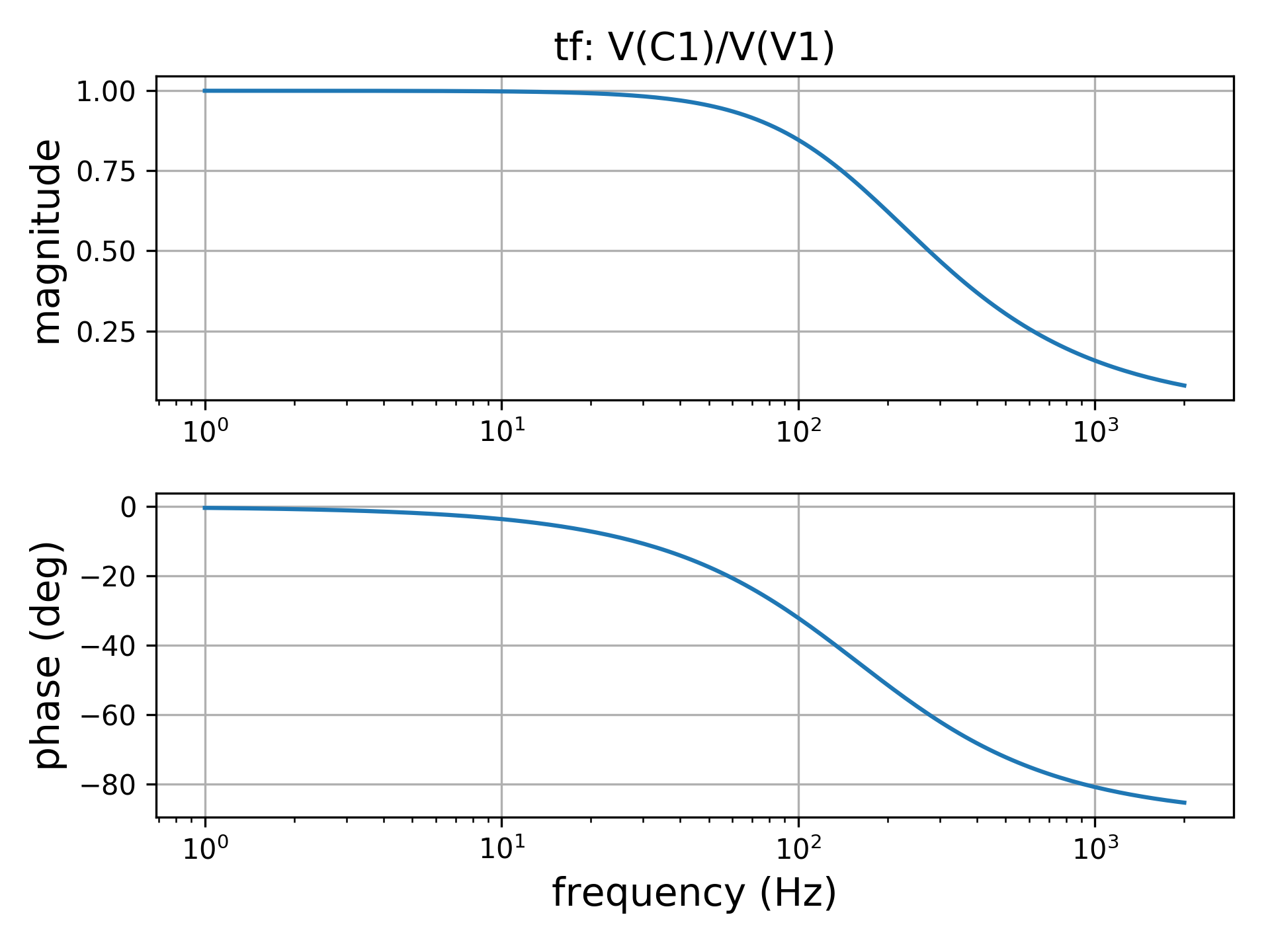
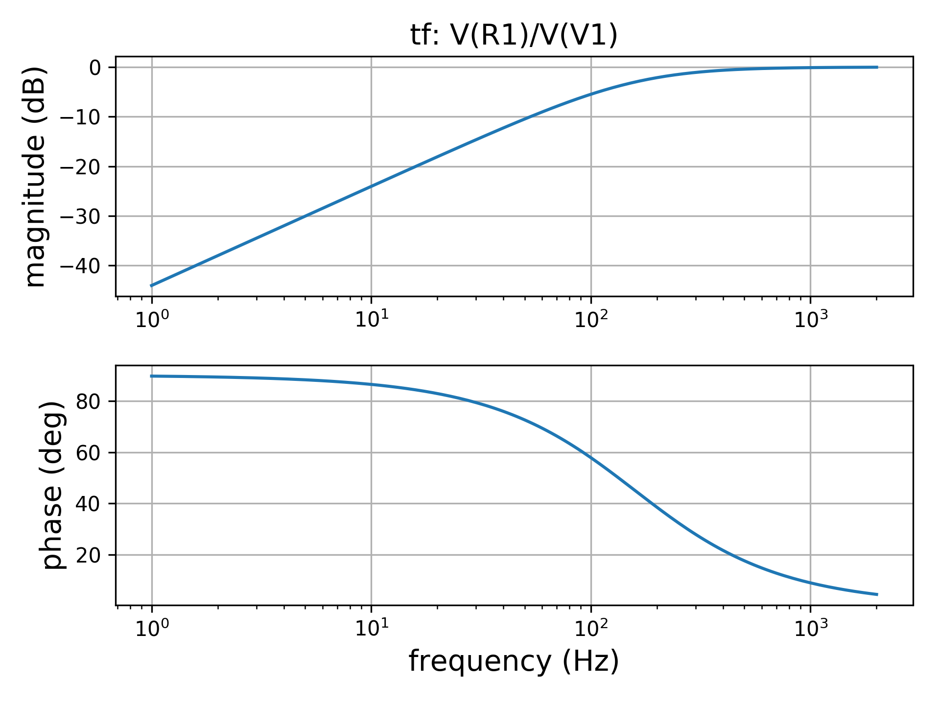
The default behaviour of net.bode() provides magnitude not in dB and phase in deg. To have the magnitude in dB one have to use the following instruction:

net.bode(decibel=True)

In this case we have:

All the above figures can be saved to a png file seting also the dpi using this instruction:

net.bode(to_file=True,filename='name_of_my_file.png',dpi_value=300)
# (decibel=True for magnitude in dB)

Band-pass filter

Let us consider the network in the following figure,

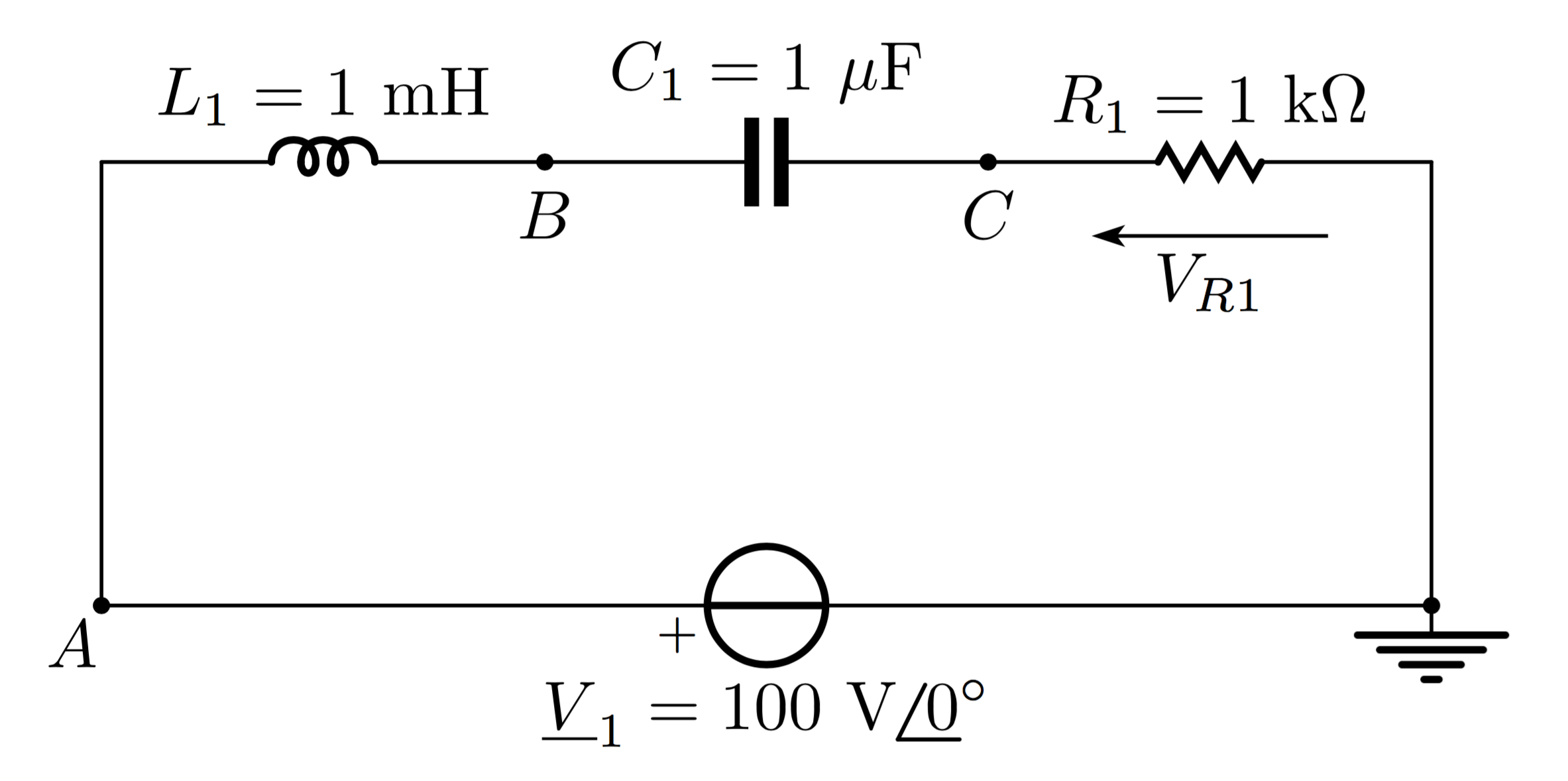
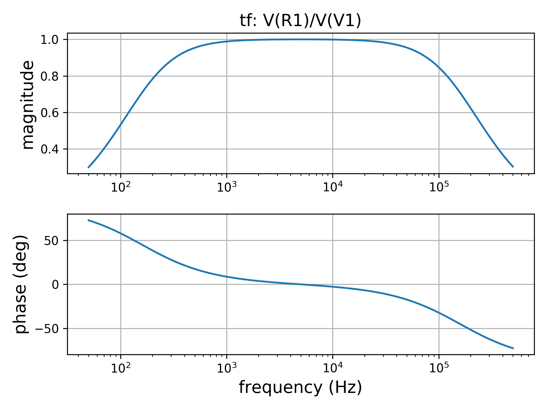
by considering the voltage across the resistor with reference to to voltage source we have a band pass filter. The resonance frequency of the circuit is fc = 1 / (2 pi sqrt(L1 C1)) = 5032.92 Hz . We are going to analyze the frequency response of the network in the range 50 Hz - 500 kHz.

The circuit can be described by the file network.net including the following lines:

* Example of AC analysis (band pass filter)
V1 A 0 100
L1 A B 1m
C1 B C 1u
R1 C 0 1k

* RC network with fc = 1/(2*pi*sqrt(L1*C1))= 5032.92 Hz

* from 1 Hz to 200 Hz with 50 points per decade
.ac dec 50 50 500k

* V(R1)/V(V1) --> band pass filter
.tf v(R1) v(V1)

Some remarks before going ahed:

.ac dec 50 50 500k run a frequency analysis from 50 Hz to 500 kHz with 50 points per decade,
the command .tf v(R1) v(V1) defines the transfer functions v(R1)/v(V1) (band-pass filter) which later will be plotted.

The same code used in the previous example provides the following bode diagram.

(without dB)

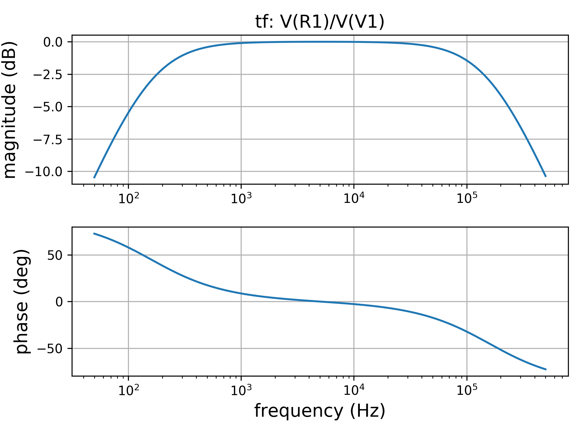
(with dB)

Transient analysis

First order circuit

Let us analyse the circuit with only one dynamic component shown below:

The circuit can be described by the file network.net including the following lines:

* Example of transient analysis
I1 0 1 8
R1 1 0 5
R2 1 2 5
L1 2 0 2m
.tran 1u 1.2m
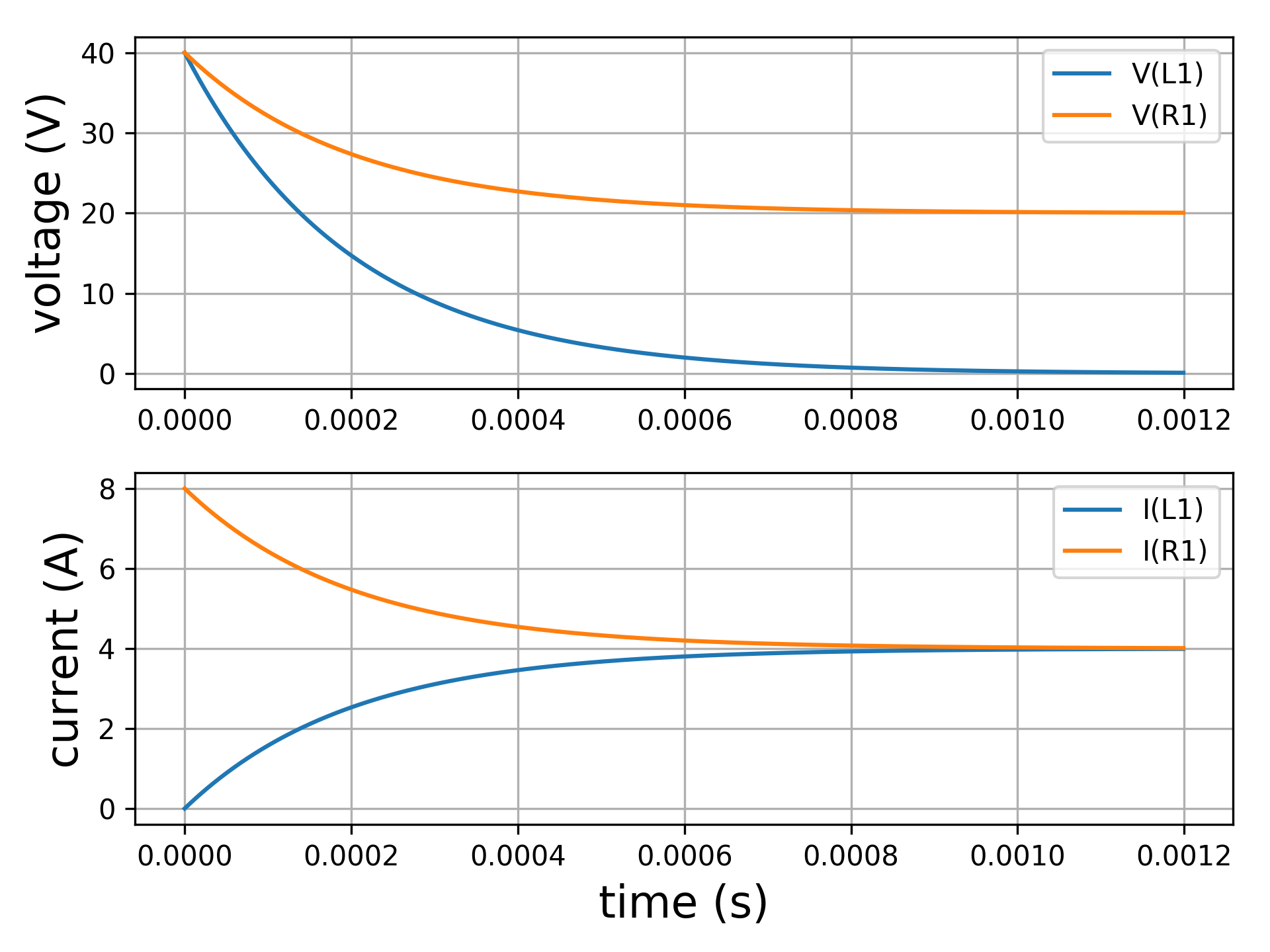
.plot v(L1) i(L1) v(R1) i(R1)

Some remarks before going ahed:

Since L1 is declared without initial condition it will be automatically considered zero
.tran 1u 1.2m means that the transient is analyzed from zero to 1.2 millisecond with time step 1 microsecond
.plot v(L1) i(L1) v(R1) i(R1) will say to SpicePy that we want the plot of the voltage and current related to L1 and R1

The network can be solved executing the following python code:

# import SciPy modules
import spicepy.netlist as ntl
from spicepy.netsolve import net_solve

# read netlist
net = ntl.Network('network.net')

# compute the circuit solution
net_solve(net)

# plot results
net.plot()

The last line of code provides the following plot:

Let us now assume we want to consider an initial condition for the inductor equal to 8 A (this means no current in R1 at t = 0 s). The netlist must be changed as given below:

* Example of transient analysis
I1 0 1 8
R1 1 0 5
R2 1 2 5
L1 2 0 2m ic=8 ; inductors with initial condition
.tran 1u 1.2m
.plot v(L1) i(L1) v(R1) i(R1)

The same code presented above provides now the following result

Second order circuit

Let us analyse the RLC circuit supplied by a constant voltage generator through a switch (image below).

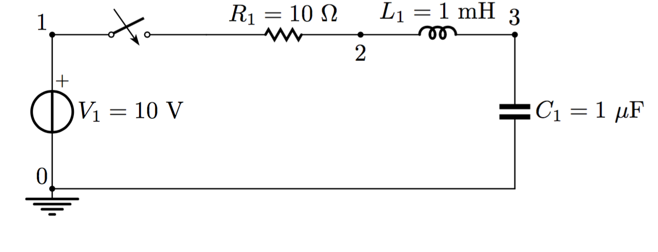
The circuit can be described by the file network.net including the following lines:

* Example of transient analysis
V1 1 0 10
R1 1 2 10
L1 2 3 1m
C1 3 0 1u
.tran 1u 1m
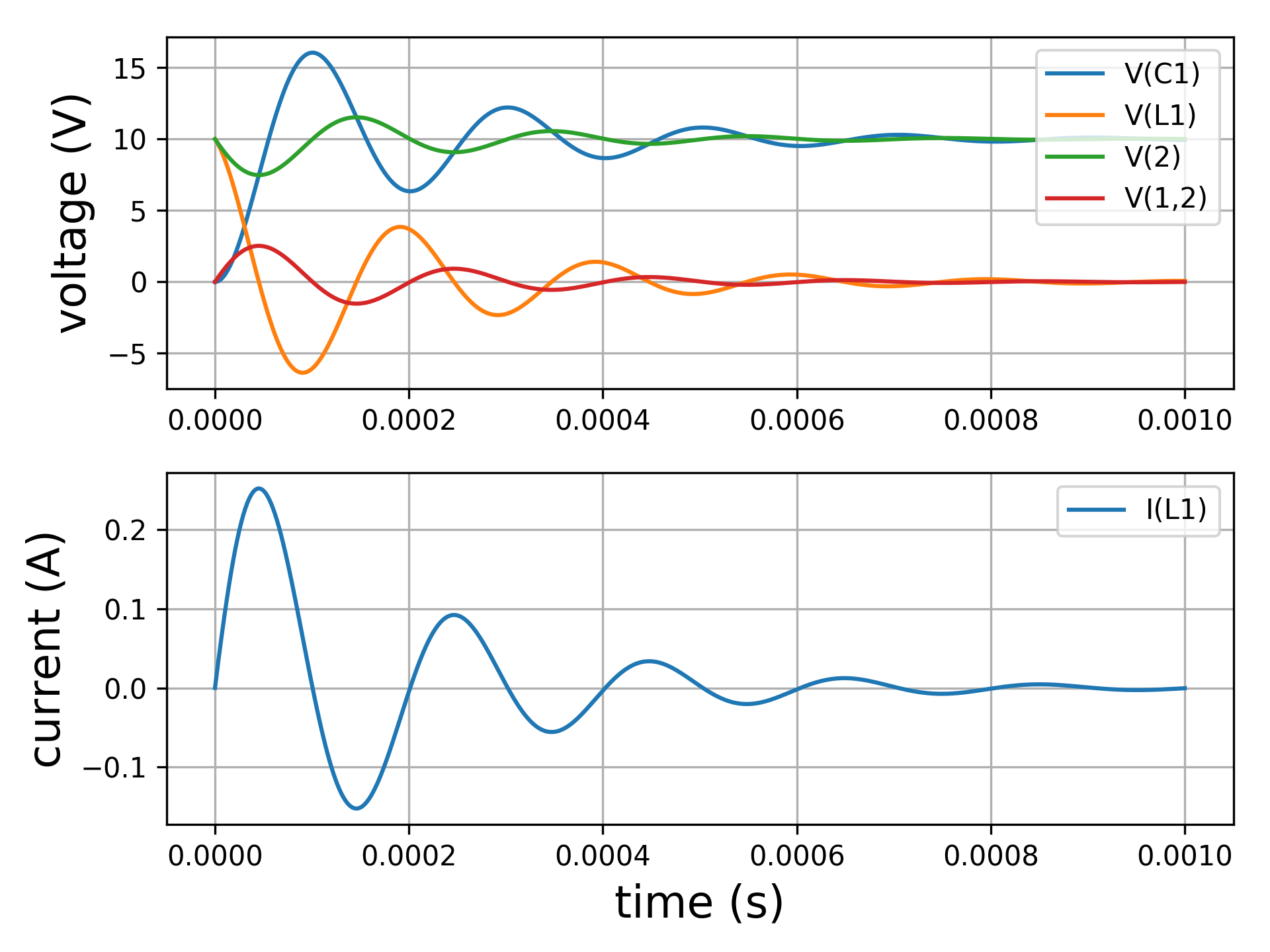
.plot v(C1) v(L1) i(L1) v(2) v(1,2)

Some remarks before going ahed:

Since L1 and C1 are declared without initial condition it will be automatically considered zero
.tran 1u 1m means that the transient is analyzed from zero to 1 millisecond with time step 1 microsecond
.plot v(C1) v(L1) i(L1) v(2) v(1,2) will say to SpicePy that we want the plot of the voltage across C1 and L1 and the current in L1 (that is equal to the current in all the other components because of the series connection among them). Furthermore v(2) is the voltage between node 2 and 0 and v(1,2) is the voltage between node 1 and 2.

The same code presented above for the 1st order circuit provides the following result:

Let us now assume we want to consider an initial condition for the capacitor equal to - 10 V. The netlist must be changed as given below:

* Example of transient analysis
V1 1 0 10
R1 1 2 10
L1 2 3 1m        ; no initial condition is equivalent to ic=0
C1 3 0 1u ic=-10 ; capacitor with initial condition
.tran 1u 1m
.plot v(C1) v(L1) i(L1) v(2) v(1,2)

If it is desired to save the output on a png file setting also the dpi, the last line of code can be changed in this way:

net.plot(to_file=True,filename='name_of_my_file.png',dpi_value=300)

In this case the following plot is also saved on the file name_of_my_file.png.

Transient input: `PULSE` (RL)

Let us analyse the RL circuit (image below) supplied by a periodic square waveform. For a complete description of the PULSE generator please refer to the documentation.

The circuit can be described by the file network.net including the following lines:

* Example of PULSE source
I1 0 1 pulse(-5 5 0 10u 10u 2.5m 5m)
R1 1 0 2
L1 1 0 1m
.tran 10u 15m
.plot i(I1) i(L1)
.end

Some remarks before going ahed:

I1 0 1 pulse(-5 5 0 10u 10u 2.5m 5m) is the square periodic waveform a(t) represented in the figure above
Since L1 is declared without initial condition it will be automatically considered zero
.tran 10u 15m means that the transient is analyzed from zero to 15 millisecond with time step 10 microsecond
.plot i(I1) i(L1) will say to SpicePy that we want the plot of source current a(t) and the current in L1.

The same code presented above for the 1st order circuit provides the following result:

Transient input: `PULSE` (RLC)

Let us analyse the RLC circuit (image below) supplied by a periodic square waveform. For a complete description of the PULSE generator please refer to the documentation.

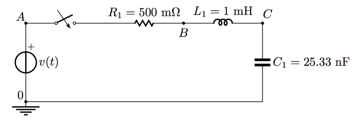
The circuit can be described by the file network.net including the following lines:

* Example of pulse source
V1 A 0 pulse(-1 1 0 5n 5n 10u 20u)
R1 A B 500m
L1 B C 1u
C1 C 0 25.33n
.tran 5n 30u
.plot v(A) v(C)

Some remarks before going ahed:

V1 A 0 pulse(-1 1 0 5n 5n 10u 20u) is the square periodic waveform v(t) represented in the figure above
Since L1 is declared without initial condition it will be automatically considered zero
.tran 5n 30u means that the transient is analyzed from zero to 30 microsecond with time step 5 nanosecond
.plot v(A) v(C) will say to SpicePy that we want the plot the potential at A and C. These potentials correspond to the source voltage and the voltage across the capacitor C1.

The same code presented above for the 1st order circuit provides the following result:

Transient input: `SIN`

Let us analyse the RL circuit (image below) supplied by a sinusoidal waveform at 50 Hz. For a complete description of the SIN generator please refer to the documentation.

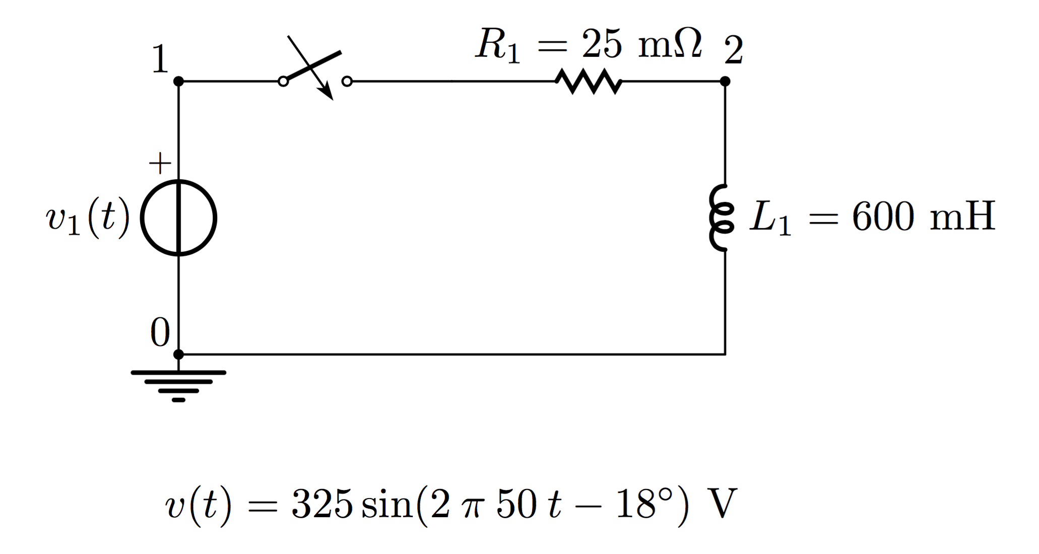
The circuit can be described by the file network.net including the following lines:

* Example of SIN source
V1 1 0 sin(0 325 50 0 0 -18)
R1 1 2 25m
L1 2 0 1m
.tran 100u 600m
.plot v(V1) i(L1)
.end

Some remarks before going ahed:

V1 1 0 sin(0 325 50 0 0 -18) is the sine wave v(t) represented in the figure above
Since L1 is declared without initial condition it will be automatically considered zero
.tran 100u 600m means that the transient is analyzed from zero to 600 millisecond with time step 100 microsecond
.plot v(V1) i(L1) will say to SpicePy that we want the plot of source voltage v1(t) and the current in L1.

The same code presented above for the 1st order circuit provides the following result:

Controlled sources: `VCVS and CCCS`

The folowing controlled sources are included in this example:

one voltage controlled voltage source (VCVS)
one current controlled current source (CCCS)

VCVSs are described in the netlist by the letter E with the following notation:

E<X>  <node+>  <node->  <nodeC+>  <nodeC->  <value>

where:

in E<X>, X is an identification number,
<node+> is one node to which the component is connected. The sign + indicates that it is conventionally the positive node. It can be either a number or a letter,
<node-> is one node to which the component is connected. The sign - indicates that it is conventionally the negative node. It can be either a number or a letter,
<nodeC+> is the conventionally positive control node. It can be either a number or a letter,
<nodeC-> is the conventionally negative control node. It can be either a number or a letter,
<value> is the voltage gain

CCCSs are described in the netlist by the letter F with the following notation:

F<X>  <node+>  <node->  <vname>  <value>

where:

in F<X>, X is an identification number,
<node+> is one node to which the component is connected. The sign + indicates that it is conventionally the positive node. It can be either a number or a letter,
<node-> is one node to which the component is connected. The sign - indicates that it is conventionally the negative node. It can be either a number or a letter,
<vname> is the name of a voltage source through which the controlling current flows.
<value> is the current gain

Let us analyse the following circuit including two controlled sources:

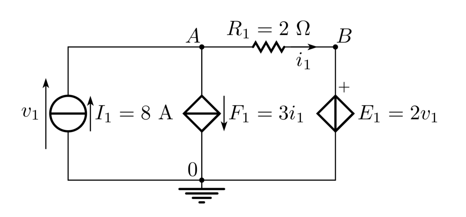
The circuit can be described by the file network.net including the following lines:

* VCVS and CCCS
F1 A 0 E1 3
E1 B 0 A 0 2
R1 B A 2
I1 0 A 8
.op

One remark before going ahed:

current-controlled sources require a voltage source to sense the control current. All kinds of voltage sources can be used. In this example the VCVS is used

The same code to solve the DC network here provides on the terminal/shell the following result is obtained:

==============================================
               branch quantities
==============================================
v(R1) =         -4 V
i(R1) =         -2 A
p(R1) =          8 W
----------------------------------------------
v(I1) =          4 V
i(I1) =          8 A
p(I1) =         32 W
----------------------------------------------
v(E1) =         -8 V
i(E1) =          2 A
p(E1) =        -16 W
----------------------------------------------
v(F1) =         -4 V
i(F1) =          6 A
p(F1) =        -24 W
----------------------------------------------

Controlled sources: `VCCS and CCVS`

The folowing controlled sources are included in this example:

one voltage controlled current source (VCCS)
one current controlled voltage source (CCVS)

VCCSs are described in the netlist by the letter G with the following notation:

G<X>  <node+>  <node->  <nodeC+>  <nodeC->  <value>

where:

in G<X>, X is an identification number,
<node+> is one node to which the component is connected. The sign + indicates that it is conventionally the positive node. It can be either a number or a letter,
<node-> is one node to which the component is connected. The sign - indicates that it is conventionally the negative node. It can be either a number or a letter,
<nodeC+> is the conventionally positive control node. It can be either a number or a letter,
<nodeC-> is the conventionally negative control node. It can be either a number or a letter,
<value> is the transconductance (siemens)

CCVSs are described in the netlist by the letter H with the following notation:

H<X>  <node+>  <node->  <vname>   <value>

where:

in H<X>, X is an identification number,
<node+> is one node to which the component is connected. The sign + indicates that it is conventionally the positive node. It can be either a number or a letter,
<node-> is one node to which the component is connected. The sign - indicates that it is conventionally the negative node. It can be either a number or a letter,
<vname> is the name of a voltage source through which the controlling current flows.
<value> is the transresistance (ohm)

Let us analyse the following circuit including two controlled sources:

The circuit can be described by the file network.net including the following lines:

* VCCS and CCVS
V1 A 0 10
R2 B C 5
G1 C B A B 2.6
R1 B A 1
R3 C 0 1
H1 D 0 V1 3
R4 E D 2
R5 E 0 4
I1 0 E 4.5
.op

The same code to solve the DC network here provides on the terminal/shell the following result is obtained:

==============================================
               branch quantities
==============================================
v(R1) =       -0.5 V
i(R1) =       -0.5 A
p(R1) =       0.25 W
----------------------------------------------
v(R2) =          9 V
i(R2) =        1.8 A
p(R2) =       16.2 W
----------------------------------------------
v(R3) =        0.5 V
i(R3) =        0.5 A
p(R3) =       0.25 W
----------------------------------------------
v(R4) =        6.5 V
i(R4) =       3.25 A
p(R4) =      21.12 W
----------------------------------------------
v(R5) =          5 V
i(R5) =       1.25 A
p(R5) =       6.25 W
----------------------------------------------
v(V1) =         10 V
i(V1) =       -0.5 A
p(V1) =         -5 W
----------------------------------------------
v(I1) =         -5 V
i(I1) =        4.5 A
p(I1) =      -22.5 W
----------------------------------------------
v(G1) =         -9 V
i(G1) =        1.3 A
p(G1) =      -11.7 W
----------------------------------------------
v(H1) =       -1.5 V
i(H1) =       3.25 A
p(H1) =     -4.875 W
----------------------------------------------

Home

Provide feedback

Saved searches

Use saved searches to filter your results more quickly

Examples

Learning by means of examples

DC network

Operating point analysis

AC analysis

Single frequency analysis

Low and high pass filter

Band-pass filter

Transient analysis

First order circuit

Second order circuit

Transient input: `PULSE` (RL)

Transient input: `PULSE` (RLC)

Transient input: `SIN`

Controlled sources: `VCVS and CCCS`

Controlled sources: `VCCS and CCVS`

Clone this wiki locally

Examples

Learning by means of examples

DC network

Operating point analysis

AC analysis

Single frequency analysis

Low and high pass filter

Band-pass filter

Transient analysis

First order circuit

Second order circuit

Transient input: PULSE (RL)

Transient input: PULSE (RLC)

Transient input: SIN

Controlled sources: VCVS and CCCS

Controlled sources: VCCS and CCVS

Clone this wiki locally

Transient input: `PULSE` (RL)

Transient input: `PULSE` (RLC)

Transient input: `SIN`

Controlled sources: `VCVS and CCCS`

Controlled sources: `VCCS and CCVS`