Dec 29, 2020
- Introduction
- Where to get help
- 1 Support Vector Machines
- 2 Spam Classification
- Submission and Grading
This programming exercise instruction was originally developed and written by Prof. Andrew Ng as part of his machine learning course on Coursera platform. I have adapted the instruction for R language, so that its users, including myself, could also take and benefit from the course.
In this exercise, you will be using support vector machines (SVMs) to
build a spam classifier. Before starting on the programming exercise, we
strongly recommend watching the video lectures and completing the review
questions for the associated topics. To get started with the exercise,
you will need to download the starter code and unzip its contents to the
directory where you wish to complete the exercise. If needed, use the
setwd() function in R to change to this directory before starting this
exercise.
Files included in this exercise
-
ex6.R- R script for the first half of the exercise -
ex6data1.Rda- Example Dataset 1 -
ex6data2.Rda- Example Dataset 2 -
ex6data3.Rda- Example Dataset 3 -
svmTrain.R- SVM rraining function -
svmPredict.R- SVM prediction function -
plotData.R- Plot 2D data -
visualizeBoundaryLinear.R- Plot linear boundary -
visualizeBoundary.R- Plot non-linear boundary -
linearKernel.R- Linear kernel for SVM - [⋆]
gaussianKernel.R- Gaussian kernel for SVM - [⋆]
dataset3Params.R- Parameters to use for Dataset 3 -
ex6_spam.R- R script for the second half of the exercise -
spamTrain.Rda- Spam training set -
spamTest.Rda- Spam test set -
emailSample1.txt- Sample email 1 -
emailSample2.txt- Sample email 2 -
spamSample1.txt- Sample spam 1 -
spamSample2.txt- Sample spam 2 -
vocab.txt- Vocabulary list -
getVocabList.R- Load vocabulary list -
readFile.R- Reads a file into a character string -
submit.R- Submission script that sends your solutions to our servers - [⋆]
processEmail.R- Email preprocessing - [⋆]
emailFeatures.R- Feature extraction from emails
⋆ indicates files you will need to complete
Throughout the exercise, you will be using the script ex6.R. These
scripts set up the dataset for the problems and make calls to functions
that you will write. You are only required to modify functions in other
files, by following the instructions in this assignment.
The exercises in this course use R, a high-level programming language
well-suited for numerical computations. If you do not have R installed,
please download a Windows installer from
R-project website.
R-Studio is a free and
open-source R integrated development environment (IDE) making R script
development a bit easier when compared to the R’s own basic GUI. You may
start from the .Rproj (a R-Studio project file) in each exercise
directory. At the R command line, typing help followed by a function
name displays documentation for that function. For example,
help('plot') or simply ?plot will bring up help information for
plotting. Further documentation for R functions can be found at the R
documentation pages.
In the first half of this exercise, you will be using support vector
machines (SVMs) with various example 2D datasets. Experimenting with
these datasets will help you gain an intuition of how SVMs work and how
to use a Gaussian kernel with SVMs. In the next half of the exercise,
you will be using support vector machines to build a spam classifier.
The provided script, ex6.R, will help you step through the first half
of the exercise.
We will begin by with a 2D example dataset which can be separated by a
linear boundary. The script ex6.R will plot the training data (Figure
1). In this dataset, the positions of the positive examples (indicated
with +) and the negative examples (indicated with o) suggest a natural
separation indicated by the gap. However, notice that there is an
outlier positive example + on the far left at about
 . As part of this exercise, you will also see how
this outlier affects the SVM decision boundary.
. As part of this exercise, you will also see how
this outlier affects the SVM decision boundary.

Figure 1: Example Dataset 1
In this part of the exercise, you will try using different values of the
 parameter with SVMs. Informally, the
parameter is a positive value that controls the
penalty for misclassified training examples. A large
parameter tells the SVM to try to classify all
the examples correctly. plays a role similar to
parameter with SVMs. Informally, the
parameter is a positive value that controls the
penalty for misclassified training examples. A large
parameter tells the SVM to try to classify all
the examples correctly. plays a role similar to
 , where
  is the
regularization parameter that we were using previously for logistic
regression.
is the
regularization parameter that we were using previously for logistic
regression.
 (Example Dataset 1)](6/tmp_files/figure-gfm/unnamed-chunk-2-1.png)
Figure 2: SVM Decision Boundary with  (Example
Dataset 1)
(Example
Dataset 1)
 (Example Dataset 1)](6/tmp_files/figure-gfm/unnamed-chunk-3-1.png)
Figure 3: SVM Decision Boundary with  (Example
Dataset 1)
(Example
Dataset 1)
The next part in ex6.R will run the SVM training (with
) using SVM software that we have included with
the starter code, svmTrain.R.[1] When , you
should find that the SVM puts the decision boundary in the gap between
the two datasets and misclassifies the data point on the far left
(Figure 2).
Implementation Note: Most SVM software packages (including
svmTrain.R) automatically add the extra feature  for you and automatically take care of learning the intercept term
 . So when passing your training data to the SVM
software, there is no need to add this extra feature
yourself. In particular, in R your code should be
working with training examples
. So when passing your training data to the SVM
software, there is no need to add this extra feature
yourself. In particular, in R your code should be
working with training examples  (rather than
 ); for example, in the first example dataset
 .
.
Your task is to try different values of on this
dataset. Specifically, you should change the value of
in the script to and run
the SVM training again. When , you should find
that the SVM now classifies every single example correctly, but has a
decision boundary that does not appear to be a natural fit for the data
(Figure 3).
In this part of the exercise, you will be using SVMs to do non-linear classification. In particular, you will be using SVMs with Gaussian kernels on datasets that are not linearly separable.
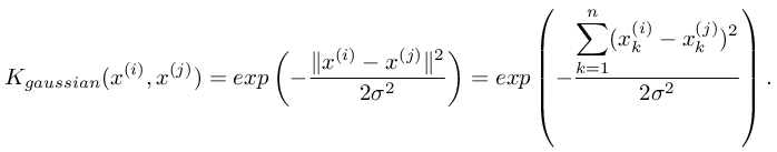
To find non-linear decision boundaries with the SVM, we need to first
implement a Gaussian kernel. You can think of the Gaussian kernel as a
similarity function that measures the “distance” between a pair of
examples, (x(i), x(j)). The Gaussian kernel is also parameterized by a
bandwidth parameter,  , which determines how fast
the similarity metric decreases (to 0) as the examples are further
apart. You should now complete the code in
, which determines how fast
the similarity metric decreases (to 0) as the examples are further
apart. You should now complete the code in gaussianKernel.R to compute
the Gaussian kernel between two examples, (x(i), x(j)). The Gaussian
kernel function is defined as:
Once you’ve completed the function gaussianKernel.R, the script
ex6.R will test your kernel function on two provided examples and you
should expect to see a value of  .
.
You should now submit your solutions.

Figure 4: Example Dataset 2
The next part in ex6.R will load and plot dataset 2 (Figure 4). From
the figure, you can obserse that there is no linear decision boundary
that separates the positive and negative examples for this dataset.
However, by using the Gaussian kernel with the SVM, you will be able to
learn a non-linear decision boundary that can perform reasonably well
for the dataset. If you have correctly implemented the Gaussian kernel
function, ex6.R will proceed to train the SVM with the Gaussian kernel
on this dataset.

Figure 5: SVM (Gaussian Kernel) Decision Boundary (Example Dataset 2)
Figure 5 shows the decision boundary found by the SVM with a Gaussian kernel. The decision boundary is able to separate most of the positive and negative examples correctly and follows the contours of the dataset well.
In this part of the exercise, you will gain more practical skills on how
to use a SVM with a Gaussian kernel. The next part of ex6.R will load
and display a third dataset (Figure 6). You will be using the SVM with
the Gaussian kernel with this dataset.

Figure 6: Example Dataset 3
In the provided dataset, ex6data3.Rda, you are given the variables X, y, Xval, yval. The provided code in ex6.R trains the SVM classifier
using the training set (X, y) using parameters loaded from
dataset3Params.R. Your task is to use the cross validation set Xval, yval to determine the best and
parameter to use. You should write any
additional code necessary to help you search over the parameters
and . For both
and , we suggest trying
values in multiplicative steps (e.g.,  ). Note
that you should try all possible pairs of values for
and (e.g.,
). Note
that you should try all possible pairs of values for
and (e.g.,
 and
and  ). For example, if you
try each of the 8 values listed above for and
for
). For example, if you
try each of the 8 values listed above for and
for  , you would end up training and evaluating (on
the cross validation set) a total of
, you would end up training and evaluating (on
the cross validation set) a total of  different
models. After you have determined the best and
parameters to use, you should modify the code in
different
models. After you have determined the best and
parameters to use, you should modify the code in
dataset3Params.R, filling in the best parameters you found. For our
best parameters, the SVM returned a decision boundary shown in Figure 7.

Figure 7: SVM (Gaussian Kernel) Decision Boundary (Example Dataset 3)
Implementation Tip: When implementing cross validation to select the
best and parameter to
use, you need to evaluate the error on the cross validation set. Recall
that for classification, the error is defined as the fraction of the
cross validation examples that were classified incorrectly. In R, you
can compute this error using mean(predictions != yval), where
predictions is a vector containing all the predictions from the SVM, and
yval are the true labels from the cross validation set. You can use the
svmPredict function to generate the predictions for the cross
validation set.
You should now submit your solutions.
Many email services today provide spam filters that are able to classify
emails into spam and non-spam email with high accuracy. In this part of
the exercise, you will use SVMs to build your own spam filter. You will
be training a classifier to classify whether a given email, x, is spam
(y = 1) or non-spam (y = 0). In particular, you need to convert each
email into a feature vector  . The following parts
of the exercise will walk you through how such a feature vector can be
constructed from an email. Throughout the rest of this exercise, you
will be using the the script
. The following parts
of the exercise will walk you through how such a feature vector can be
constructed from an email. Throughout the rest of this exercise, you
will be using the the script ex6_spam.R. The dataset included for this
exercise is based on a a subset of the SpamAssassin Public Corpus. For
the purpose of this exercise, you will only be using the body of the
email (excluding the email headers).
> Anyone knows how much it costs to host a web portal?
>
Well, it depends on how many visitors youre expecting.
This can be anywhere from less than 10 bucks a month to a couple of $100.
You should checkout http://www.rackspace.com/ or perhaps Amazon EC2
if you're running something big..
To unsubscribe yourself from this mailing list, send an email to:
[email protected]
Figure 8: Sample Email
Before starting on a machine learning task, it is usually insightful to take a look at examples from the dataset. Figure 8 shows a sample email that contains a URL, an email address (at the end), numbers, and dollar amounts. While many emails would contain similar types of entities (e.g., numbers, other URLs, or other email addresses), the specific entities (e.g., the specific URL or specific dollar amount) will be different in almost every email. Therefore, one method often employed in processing emails is to “normalize” these values, so that all URLs are treated the same, all numbers are treated the same, etc. For example, we could replace each URL in the email with the unique string “httpaddr” to indicate that a URL was present.
This has the effect of letting the spam classifier make a classification
decision based on whether any URL was present, rather than whether a
specific URL was present. This typically improves the performance of a
spam classifier, since spammers often randomize the URLs, and thus the
odds of seeing any particular URL again in a new piece of spam is very
small. In processEmail.R, we have implemented the following email
preprocessing and normalization steps:
- Lower-casing: The entire email is converted into lower case, so that captialization is ignored (e.g., IndIcaTE is treated the same as Indicate).
- Stripping HTML: All HTML tags are removed from the emails. Many emails often come with HTML formatting; we remove all the HTML tags, so that only the content remains.
- Normalizing URLs: All URLs are replaced with the text “httpaddr”.
- Normalizing Email Addresses: All email addresses are replaced with the text “emailaddr”.
- Normalizing Numbers: All numbers are replaced with the text “number”.
- Normalizing Dollars: All dollar signs ($) are replaced with the text “dollar”.
- Word Stemming: Words are reduced to their stemmed form. For example, “discount”, “discounts”, “discounted” and “discounting” are all replaced with “discount”. Sometimes, the Stemmer actually strips off additional characters from the end, so “include”, “includes”, “included”, and “including” are all replaced with “includ”.
- Removal of non-words: Non-words and punctuation have been removed. All white spaces (tabs, newlines, spaces) have all been trimmed to a single space character.
The result of these preprocessing steps is shown in Figure 9. While preprocessing has left word fragments and non-words, this form turns out to be much easier to work with for performing feature extraction.
anyon know how much it cost to host a web portal well it depend on how
mani visitor your expect thi can be anywher from less than number buck
a month to a coupl of dollarnumb you should checkout httpaddr or perhap
amazon ecnumb if your run someth big to unsubscrib yourself from thi
mail list send an email to emailaddr
Figure 9: Preprocessed Sample Email
1 aa
2 ab
3 abil
...
86 anyon
...
916 know
...
1898 zero
1899 zip
Figure 10: Vocabulary List
86 916 794 1077 883
370 1699 790 1822
1831 883 431 1171
794 1002 1893 1364
592 1676 238 162 89
688 945 1663 1120
1062 1699 375 1162
479 1893 1510 799
1182 1237 810 1895
1440 1547 181 1699
1758 1896 688 1676
992 961 1477 71 530
1699 531
Figure 11: Word Indices for Sample Email
After preprocessing the emails, we have a list of words (e.g., Figure 9)
for each email. The next step is to choose which words we would like to
use in our classifier and which we would want to leave out. For this
exercise, we have chosen only the most frequently occuring words as our
set of words considered (the vocabulary list). Since words that occur
rarely in the training set are only in a few emails, they might cause
the model to overfit our training set. The complete vocabulary list is
in the file vocab.txt and also shown in Figure 10. Our vocabulary list
was selected by choosing all words which occur at least a 100 times in
the spam corpus, resulting in a list of 1899 words. In practice, a
vocabulary list with about 10,000 to 50,000 words is often used. Given
the vocabulary list, we can now map each word in the preprocessed emails
(e.g., Figure 9) into a list of word indices that contains the index of
the word in the vocabulary list. Figure 11 shows the mapping for the
sample email. Specifically, in the sample email, the word “anyone” was
first normalized to “anyon” and then mapped onto the index 86 in the
vocabulary list.
Your task now is to complete the code in processEmail.R to perform
this mapping. In the code, you are given a string str which is a single
word from the processed email. You should look up the word in the
vocabulary list vocabList and find if the word exists in the vocabulary
list. If the word exists, you should add the index of the word into the
word indices variable. If the word does not exist, and is therefore not
in the vocabulary, you can skip the word. Once you have implemented
processEmail.R, the script ex6_spam.R will run your code on the
email sample and you should see an output similar to Figures 9 & 11.
R Tip: In R, you can compare two strings with the == infix
function. For example, str1==str2 will return TRUE only when both
strings are equal. In the provided starter code, vocabList is a R’s
“character vector” containing the words in the vocabulary. In R, you
index into them using square brackets. Specifically, to get the word at
index i, you can use vocabList[i]. You can also use
length(vocabList) to get the number of words in the vocabulary.
You should now submit your solutions.
You will now implement the feature extraction that converts each email
into a vector in  . For this exercise, you will be
using
. For this exercise, you will be
using  words in vocabulary list. Specifically, the
feature
words in vocabulary list. Specifically, the
feature  for an email corresponds to whether the
 -th word in the dictionary occurs in the email.
That is,
-th word in the dictionary occurs in the email.
That is,  if the -th word
is in the email and
if the -th word
is in the email and  if the
-th word is not present in the email. Thus, for a
typical email, this feature would look like:
if the
-th word is not present in the email. Thus, for a
typical email, this feature would look like:

You should now complete the code in emailFeatures.R to generate a
feature vector for an email, given the word indices. Once you have
implemented emailFeatures.R, the next part of ex6_spam.R will run
your code on the email sample. You should see that the feature vector
had length  and
and  non-zero
entries.
non-zero
entries.
You should now submit your solutions.
After you have completed the feature extraction functions, the next step
of ex6_spam.R will load a preprocessed training dataset that will be
used to train a SVM classifier. spamTrain.Rda contains 4000 training
examples of spam and non-spam email, while spamTest.Rda contains 1000
test examples. Each original email was processed using the processEmail
and emailFeatures functions and converted into a vector
 . After loading the dataset,
 ex6_spam.R will
proceed to train a SVM to classify between spam  and non-spam
  emails. Once the training
completes, you should see that the classifier gets a training accuracy
of about 99.8% and a test accuracy of about 98.5%.
emails. Once the training
completes, you should see that the classifier gets a training accuracy
of about 99.8% and a test accuracy of about 98.5%.
our click remov guarante visit basenumb dollar will price pleas nbsp most lo ga dollarnumb
Figure 12: Top predictors for spam email
To better understand how the spam classifier works, we can inspect the
parameters to see which words the classifier thinks are the most
predictive of spam. The next step of ex6_spam.R finds the parameters
with the largest positive values in the classifier and displays the
corresponding words (Figure 12). Thus, if an email contains words such
as “guarantee”, “remove”, “dollar”, and “price” (the top predictors
shown in Figure 12), it is likely to be classified as spam.
Now that you have trained a spam classifier, you can start trying it out
on your own emails. In the starter code, we have included two email
examples (emailSample1.txt and emailSample2.txt) and two spam
examples (spamSample1.txt and spamSample2.txt). The last part of
ex6_spam.R runs the spam classifier over the first spam example and
classifies it using the learned SVM. You should now try the other
examples we have provided and see if the classifier gets them right. You
can also try your own emails by replacing the examples (plain text
files) with your own emails.
You do not need to submit any solutions for this optional (ungraded) exercise.
In this exercise, we provided a preprocessed training set and test set.
These datasets were created using the same functions (processEmail.R
and emailFeatures.m) that you now have completed. For this optional
(ungraded) exercise, you will build your own dataset using the original
emails from the SpamAssassin Public Corpus. Your task in this optional
(ungraded) exercise is to download the original files from the public
corpus and extract them. After extracting them, you should run the
processEmail [2] and emailFeatures functions on each email to extract
a feature vector from each email. This will allow you to build a dataset
X, y of examples. You should then randomly divide up the dataset into a
training set, a cross validation set and a test set. While you are
building your own dataset, we also encourage you to try building your
own vocabulary list (by selecting the high frequency words that occur in
the dataset) and adding any additional features that you think might be
useful. Finally, we also suggest trying to use highly optimized SVM
toolboxes such as LIBSVM.
You do not need to submit any solutions for this optional (ungraded) exercise.
After completing various parts of the assignment, be sure to use the submit function system to submit your solutions to our servers. The following is a breakdown of how each part of this exercise is scored.
| Part | Submitted File | Points |
|---|---|---|
| Gaussian Kernel | gaussianKernel.R |
25 points |
| Parameters (, ) for Dataset 3 |
dataset3Params.R |
25 points |
| Email Preprocessing | processEmail.R |
25 points |
| Email Feature Extraction | emailFeatures.R |
25 points |
| Total Points | 100 points |
You are allowed to submit your solutions multiple times, and we will take only the highest score into consideration.
-
In order to ensure compatibility with R, we have included this implementation of an SVM learning algorithm. However, this particular implementation was chosen to maximize compatibility, and is not very efficient. If you are training an SVM on a real problem, especially if you need to scale to a larger dataset, we strongly recommend instead using a highly optimized SVM toolbox such as LIBSVM.
-
The original emails will have email headers that you might wish to leave out. We have included code in processEmail that will help you remove these headers.