Here are some elapsed times (in s) for 4 implementations.
| # particles | Py | C++ | Fortran | Julia |
|---|---|---|---|---|
| 1024 | 29 | 55 | 41 | 45 |
| 2048 | 123 | 231 | 166 | 173 |
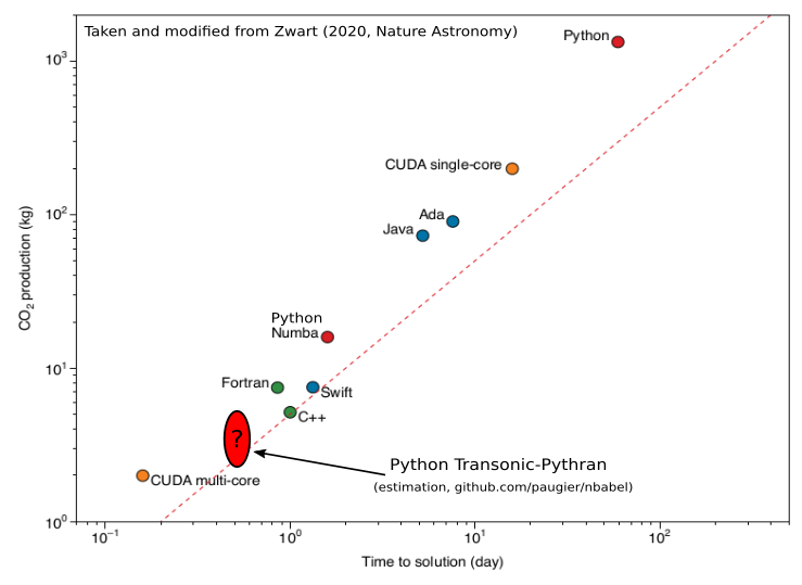
The implementations in C++, Fortran and Julia come from https://www.nbabel.org/ and have recently been used in an article published in Nature Astronomy (Zwart, 2020). The implementation in Python-Numpy is very simple, but uses Transonic and Pythran.
To run these benchmarks, go into the different directories and run make bench1k or make bench2k.
To give an idea of what it gives compared to the figure published in Nature Astronomy:
Note: these benchmarks are run sequentially with a Intel(R) Core(TM) i5-8400 CPU @ 2.80GHz.
Note 2: With Numba (environment variable TRANSONIC_BACKEND="numba"), the
elapsed times are 55 s and 206 s, respectively.
We can also compare different solutions in Python. Since some solutions are very slow, we need to compare on a much smaller problem (only 128 particles). Here are the elapsed times (in s):
| Transonic-Pythran | Transonic-Numba | High-level Numpy | PyPy OOP | PyPy lists |
|---|---|---|---|---|
| 0.48 | 3.91 | 686 | 87 | 15 |
For comparison, we have for this case {"c++": 0.85, "Fortran": 0.62, "Julia": 2.57}.
Note that just adding from transonic import jit to the simple high-level
Numpy code and then decorating the function compute_accelerations with
@jit, the elapsed time decreases to 8 s (a x85 speedup!, with Pythran 0.9.8).